While you can do many operations in R using data objects that contain a single data item, most of the interesting things you will want to do will involve data objects that contain multiple data items. The exercises in this learning infrastructure topic will help familiarize you with R multiple data item objects like vectors, matrices, and data frames.

Vectors

A vector, in R, is a list of data items. A vector can contain numbers, character strings, or logical values but not a mixture. All of the data items in a vector must be the same type.

Here is an example of a vector

x <- c(1, 2, 3, 4, 5, 6, 7, 8, 9, 10) # create a numeric vector

The function c( ) combines the numeric values from 1 to 10 into a vector. You can also obtain the same result using this

x <- c(1:10) # create a numeric vector

The annotation 1:10 indicates the series of values from 1 to 10. If you want to view the contents of the vector simply type x and press ENTER, R will display the data items in the vector. The vector x will appear in the RStudio Environment panel. It shows the object name [x], the object data type [int], the size of the object [1:10], and its contents [1, 2, 3, 4, 5, 6, 7, 8, 9, 10]. The Environment panel cannot show the complete contents of a very large object. This code

a <- c(x, x, x)

Will result in a vector containing 30 data items. The Environment panel shows the object name, its data type, its size, and the first set of data items followed by an ellipsis [...] indicating that there are more elements not shown.

You can easily access individual elements of a vector. You can view the 4th element in the vector using the code x[4]. This is called indexing. The value in the square braces is the index or location you want to access. You can also index multiple consecutive elements using a colon in your index notation. So x[3:6] will display the data items at the 3, 4, 5, and 6 indices of x. You can also exclude specific data items in a vector. So x[-3] will return all of the elements in x except the 3rd one and x[-(3:6)] will exclude the 3rd, 4th, 5th, and 6th elements. Notice that the 3:6 series indicator is enclosed in parenthesis. This lets R know that you intend to exclude this series. If you leave out the parenthesis, R will interpret this code as nonsense and return an error message: Error in x[-3:6] : only 0's may be mixed with negative subscripts.

R will let you easily apply an operation to the elements of a vector. The operation x + 2 adds 2 to each element of x. This operation will return a vector of the result of adding 2 to each data item in x. You can apply an operation to a subset of consecutive elements in a vector using the method shown above. The code x[3:6] + 2 will add 2 to the 3rd, 4th, 5th, and 6th elements in x. You can even use operations like x > 4. This operation will return a vector of logical values [TRUE or FALSE] resulting from comparing each data item in x to the number 4.

Before moving on to the next topic, run this code and create the following vectors.

y <- c(11:20) # create a numeric vector

z <- c(21:30) # create a numeric vector

t <- c("red", "blue", "red", "white", "blue", "white", "red","blue", "white", "white")

Now you have four vectors. The three vectors x, y, and z contain numeric values and the fourth vector t contains character strings. You can verify this using the mode( ) function. When you enter mode(x), mode(y), or mode(z), R will respond with the result "numeric". When you enter mode(t), R will respond with the result "character".

Matrices

There will be times that you will want to work with your data organized into a matrix. In R a matrix is an M x N collection of data items. They must all be of the same data type and each row and column must be the same size. You have conveniently created four vectors that you can use to create a matrix.

There are several ways to combine vectors into a matrix. Here is one technique

a <- c(x, y, z) # create a numeric vector by combining x, y, and z

m2 <- matrix(a, 10, 3) # create a matrix with 10 rows and 3 columns

Here is another technique

m1 <- cbind(x, y, z) # create a matrix by combining x, y, and z

If you enter m1 in the RStudio command console, R will respond with

       x  y  z

 [1,]  1 11 21

 [2,]  2 12 22

 [3,]  3 13 23

 [4,]  4 14 24

 [5,]  5 15 25

 [6,]  6 16 26

 [7,]  7 17 27

 [8,]  8 18 28

 [9,]  9 19 29

[10,] 10 20 30

If you enter m2 in the RStudio command console, R will respond with

          [,1] [,2] [,3]

 [2,]   2   12   22

 [3,]   3   13   23

 [4,]   4   14   24

 [5,]   5   15   25

 [6,]   6   16   26

 [7,]   7   17   27

 [8,]   8   18   28

 [9,]   9   19   29

The data items in both matrices are the same. The main difference between how the two techniques create each matrix is the column titles. In m1 the column titles are the original vector object names. In m2 the columns simply have index identifiers. This difference does not matter because the elements of a matrix are accessed by their indexes only. These column names are cannot be used to access matrix elements.

You can access the elements of a matrix using indexing. Matrix indexes are similar to vector indexes. The only difference is that you now have to identify both the row and the column index. As an example of matrix indexing, the code m1[5, 2] will return the value stored in the 5th row of the 2nd column of m1, or the value 15. You can also access entire rows, m2[3,] will return the third row of m2, or the vector 3, 13, and 23. Similarly, m1[,1] returns the 1st column of m1. The code m1[3:6, 2:3] will return a matrix containing rows 3 through 6 from columns 2 and 3 from m1.

By now it should not come as a surprise that the code m1 + 2 will output a matrix containing data items that are the result of adding 2 to each data item in m1

If you recall, this section began by describing an R matrix as an M x N collection of data items of the same data type. The code mode(m1) will get the response of "numeric". If you combine m1 and the vector t into a 10 x 4 matrix something odd occurs. You and combine these objects using the command

mx <- cbind(m1, t)

When you view the new matrix by typing mx and pressing ENTER, R will respond with

                x    y    z    t

This result may surprise you, but it makes sense when you remember that the data items in the matrix mx must be the same data type. In this case, when you combined the character vector t to m1, R forced or coerced all of the data elements into a single compatible data type. Since R could not coerce the character strings in t to become numeric values, it coerced the numeric values in m1 to become character values. You can verify this with the code mode(mx). R will respond with "character".

If your intent is to create an R data storage object that contains mixed data types, you will need to use a data frame.

Data Frames

A data frame is a powerful and flexible data structure. Most serious R applications involve data frames. A data frame is a tabular data structure, consisting of rows and columns and implemented as a list. The columns of a data frame can consist of different data types but each column must be a single data type [like a vector]. Because a data frame is, in its structure, a list, there are two ways to access the data items in the data frame. You can use indices, like you did with matrices, or you can use R list operators, like the column title dfrm$name, to access the data elements.

You can start with the matrix m1 from the exercise above and create a data frame. This code will do that

             x  y  z    t

Notice a few things about the data frame df. First, the rows are preceded with row numbers, not indices in square braces. Second, the first three columns are numeric and the fourth column is character. You can verify this with the commands: mode(df$x), mode(df$y), mode(df$z), and mode(df$t). Third, as you may have noticed in those mode( ) commands, you can identify a column of the data frame using its title instead of indexing it. In fact, as you type the data frame name and the $, you should notice that RStudio prompts you with a popup hint of the column titles that you can select from. Finally, notice that the code you used for this exercise created a data frame out of vectors of the same data type and then added the vector of a different data type.

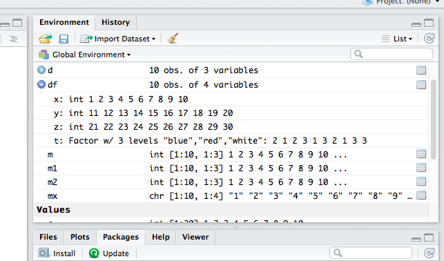
If you look in the RStudio Environment panel, you will see that the data frame df is shown differently than the other objects in the environment panel. It has an arrow before the object name. If you click that arrow, you will see more detail of the data frame's structure.

As with vectors and matrices, you can apply any R operation to a data frame within the constraints of its structure. This means that you cannot use this command

df + 2

because you cannot add 2 to the character strings in the df$t column. It does not make mathematical sense. On the other hand, the command

df[1:3] + 2

or